Working with polynomials
Create a polynomial object by clicking on the respective icon of the main menu. Before using it, the method and the learn attribute must be specified. For the learn attribute one of the samples of the project has to be selected as the training sample. The optional test attribute allows to select another sample as the test sample. Once the polynomial is fitted to the training sample the mean squared error on the training sample is shown as the residual noise attribute. If a test sample is selected, the mean squared error on the test sample will be shown as the residual test noise attribute.The method attribute allows the user to select among six options:
| manual: | specify the degree and precision of a polynomial by hand. |
| two-part MDL: | find the optimum degree by penalization. |
| mixture MDL: | by using the minimax algorithm for mixture MDL. |
| cross-validation: | to compare with the performance of the MDL methods. |
| analysis: | calculate the generalization error on a test sample. |
| complex analysis: | repeat the generalization analysis over training samples of different size. |
Using a method other than manual will open an additional plot that shows the results of the method. Clicking on the graph of the additional plot will load the polynomial into the editor, just like clicking on the polynomial in the main plot.
The manual method. The manual method was specifically added to allow the user to play with the parameters of a polynomial. You can specify the degree of a polynomial and the precision in digits per parameter. Clicking on the fit action will calculate the least square fit of the polynomial on the sample. Playing with the precision will show you the effects of rounding. Usually, for less than k/3 digits per parameter the polynomial cannot approximate the sample. The mean squared error on the training sample becomes very high. k/2 gives an almost optimum result. Higher precisions will let the mean squared error decrease only marginally.
Clicking on the precision editor attribute will allow you to specify the precision for individual parameters. A window pops up with the value and the precision of each individual parameter. The precisions can be changed and the polynomial can be fitted again, resulting in the parameters that give the best result for the specified precision.
The two-part MDL method. If you use this method or any of the other methods that calculate an optimum degree, you cannot manually change the degree or the precision of the polynomial. Rather, you specify the maximum degree that will be looked at and the method will search for the best degree. 50 to 100 degrees as a maximum are usually quite enough to work with. The rounding procedures give precise results for at least a 150 degrees but computations become awfully slow. If processor speed continues to grow at the current rate we will soon watch a 1,000 degree polynomial being fitted at a speed fast enough for direct interaction. But this will not significantly alter our results.
The penalty attribute specifies the way the total code length is calculated. The default is Rissanen's original term, as calculated in Section 2.2 of the thesis.
You can modify this term or replace it by the AIC, which is nlogσ2+2k. The penalty attribute will accept every function name that is specified in the C/C++ math libraries: log(), ln(), sin(), cos(), sqrt(), and so on. The standard operators +, -, /, *, ^ are defined. In addition, the following single letter symbols are available:
| n | the size of the sample |
| k | the degree of the polynomial |
| s | the mean squared error σ2 of the polynomial on the sample |
| p | the real number π |
| e | the real number e |
Clicking on the fit button will calculate the least square polynomial for every degree smaller than the maximum degree. The complexity is calculated according to the penalty term and immediately shown on the additional plot. Once the complexity for all degrees has been calculated, the model that had the shortest two-part complexity is selected as the good model. It is calculated and plotted into the main graph.
If you want to save time and don't want to look at every degree, specify the number of steps parameter. If it is bigger than the maximum, all degrees will be looked at. If it is smaller, only this number of degrees will be looked at. Starting at the 0/-degree polynomial and continuing to the maximum degree, superfluous degrees will be left out at equal intervals.
The mixture MDL method. The mixture MDL method works exactly like the two-part MDL method, except for the fact that no penalty term can be specified.
The cross-validation method. This method also works like the two-part MDL method without the penalty term. Future versions may allow to modify the smoothing algorithm and the number of partitions used in the algorithm.
The analysis method. This method also works like the two-part MDL method without the penalty term. But the test sample is now mandatory. Keep in mind that it should contain at least 1,000 points. Don't make it too big as this will slow down calculations. 3,000 points have been proven to be a good size for most learning problems. The optimum model according to the generalization analysis is plotted into the main plot.
The complex analysis method. This last method was not introduced during the experiments. Like the analysis method it calculates the generalization error for all degrees. But it does so for training samples of varying size. The number of samples attribute specifies how many samples are used. These samples are subsets of the selected training sample. If the training sample has 600 points and the number of samples is 20, the first set contains 30 points, the second 60, the third 90 and so on. The test sample is not changed.
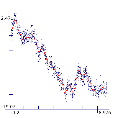
Pendulum with 600 point training set and 3,000 point test set.
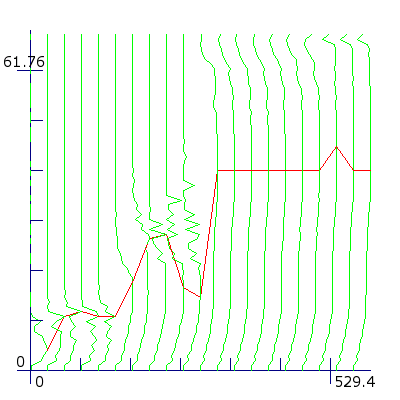
Complex analysis with 20 different samples of size 30--600 points. Each vertical line represents the generalization error for one sample, starting on the left with the smallest sample. The lower the error the more the line deviates to the right. The single horizontal line goes through all the optima. From a sample size of 330 points onwards the optimum stays almost constantly at 41 degrees.
The plot of this method is three-dimensional. The x-axis shows the sample size, the y-axis shows the degree and the z-axis shows the generalization error. The view is tilted so that a high value along the z-axis results in a shift of a point to the left. For each sample the generalization error is a vertical line along the y-axis. The lower the generalization error, the more this line goes to the right and the higher the error the more the line goes to the left. To mark the optimum number of degrees per sample size, a single horizontal line connects all the optima.
To get more reliable results for the generalization error per sample size, for small samples the average is taken over multiple samples of the same size. For sample sizes smaller than half the size of the original training sample the average is taken over two independent samples of the same size. For samples smaller than a third the average is taken over three and for samples smaller than a fourth the average is taken over four independent samples of the same size.
The complex analysis method makes it possible to study the behavior of the generalization error as a function of the size of the training set. If polynomials converge only slowly with the original problem, the optimum will rise continuously. But smooth functions like the sinus wave, the pendulum and the Lorenz attractor usually show an initial increase followed by an almost flat region.