Defining a process

Besides the standard attributes, a process has a series object that defines the type of the process, two attributes that define the beginning and the end of the range over the x-axis of the process and a make action which will create the process once its properties are defined.

Seven different processes are available as predefined two-dimensional learning problems. Most of them are common in nature. They include sinus waves, time series, fractals and the step function. Some are smooth, others have sharp corners. Some have extreme values, others deviate only slightly from the main path. Using the default parameters of a process and the random generator will generate a broad range of interesting problems. Manipulating the process specific parameters will generate an even broader variety of different problems.

Besides the process specific parameters, all processes have a system noise, a seed, a steps and a scale attribute. Because the evolution of a time series often involves some system noise, most processes depend on the random generator. The system noise must not be confused with the deviation of the points of a sample along the y-axis. It is a major factor in defining the shape of a time series. The system noise attribute defines the variance of the Gaussian distribution over this noise. Setting the seed attribute to a value other than zero will always produce the same shape for such a process.

The steps attribute defines how fast the process will evolve over the defined range of the x-axis. The default values are set in a way that most series can be approximated well by a 50 degrees polynomial. More steps will let the series evolve faster and a higher degree polynomial will be needed to learn it. The scale attribute defines the amplitude of a process along the y-axis.

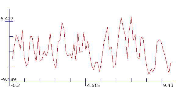
Auto-regression. Autoregressive time series are particularly common in nature. The value y_t at time y of such a series is the weighted sum

y_t = a₀ + Σⁿ_i=1 a_i y_t-i + ε
over n previous values of y. ε is the system noise. The application allows you to specify six different parameters a₀ - a₅ but three parameters is usually quite enough. The example has a₁=0.5, a₂=0.5. The other parameters are equal to zero:



Auto-regression

In all graphs of time series the horizontal x-axis shows the time t and the vertical y-axis shows the value y. If more than one value changes with time, the other values are not shown in the graph and are not used for the experiments.

Sinus wave. The sinus wave is also very common. Five frequencies can be specified, each with an individual offset. The resulting function is

f(x) = Σ⁵_i=1 sin (f_i x + o_i)

The example uses zero offsets and the four frequencies f₁=1.05, f₂=0.8, f₃=0.55 and f₄=0.15:



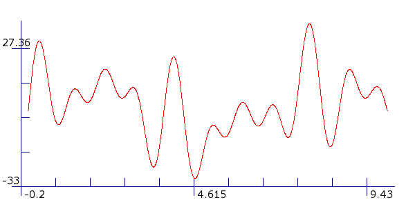
Sinus wave

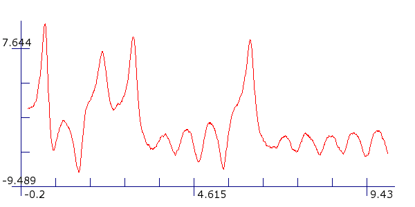
Logistic map. A logistic map is a time series of the form

y_t = a y_t-1 (1-y_t-1)+ε
with ε the system noise. It was first published by the Belgian mathematician Pierre Verhulst sometime between 1838 and 1850.

The example has a=0.5:



Logistic map

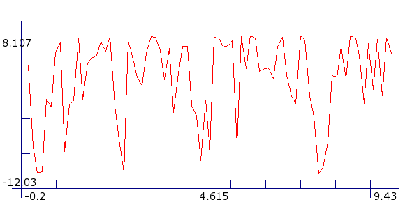
Lorenz attractor. The famous Lorenz attractor is a self similar object. It is also a time series. E.N. Lorenz discovered it when he was working on models of the weather. Its evolution is governed by the equations

y_t = a (z_t-1-y_t-1)+ε

z_t = by_t-1-z_t-1 w_t-1+ε

w_t = y_t-1 z_t-1-c y_t-1) +ε

z and w are not shown in the graph and are not considered in the experiments. The default values are a=10, b=28, c=2.667:



Lorenz attractor

Pendulum. The movement of a noisy pendulum with orbit o and frequency f is defined as

y_t = sin(y_t-2)-c y_t-1 +f cos(o (t-2)) +ε

The example has c=0.2, f=0.5 and o=0.67.



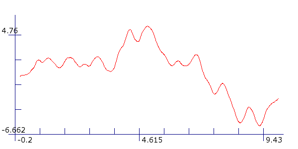
Pendulum

Step function. The step function oscillates n times between two values. The example in Figure~{figure-step-function} has n=10 and oscillates between minus ten and ten. The points where the function switches between values are chosen at random. The same non-zero seed will produce the same step function.



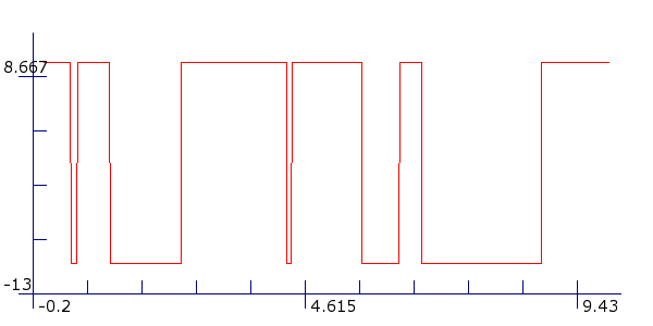
Step function

Thom map. The Thom map is also a time series. R. Thom discovered it when he searched for a simple discrete equivalent to the Lorenz equations which were defined for continous time.



y_t = a y_t-1+b z_t-1

z_t = c y_t-1+d z_t-1
z is not shown in the graph and is not considered in the experiments. The example has a=0.5, b=0.3, c=0.3 and d=0.4.



Thom map